Standard method of characteristics

Characteristics, also known as exceptional or critical initial manifolds (Courant and Hilbert, 1962), are defined as follows: if the matrix of coefficients of derivatives in a partial differential equation (PDE) is singular on a curve or surface, it is a characteristic curve or surface. Characteristics can be used to reduce the number of variables to be considered. In the special case of a first-order PDE, along the characteristics the PDE is reduced to a system of ODEs. However, such reduction in number of variables may transform a linear PDE into an equation of fewer variables. Such an equation is a nonlinear one, as we shall see later in this document. Also, an initial solution cannot be specified along a characteristic curve or surface, since, given one displacement value on such a surface, all other values are then determined so we cannot arbitrarily specify a second (or further) one.

When the method is applied to the wave equation for arbitrary inhomogeneity and elliptical velocity dependence it involves

1. ascertaining whether the determinant of a three-by-three matrix of coefficients of first derivatives is non-zero so that the system can be solved, and
2. setting the determinant of the six-by-six matrix of coefficients of second derivatives to zero to obtain the eikonal equation.

My next step is to apply the above method to find the characteristics of Cauchy's equations of motion (5) for inhomogeneous anisotropic media. The characteristic surface is one on which the second-order derivatives of $u$ cannot be determined. The first-order derivatives in equations (5) are determined from the initial conditions.

According to Bos (2003), the characteristic surface is one on which the second-order partial derivatives of $u$ cannot be determined. So let us consider a surface $S$ given in functional form by $t=f(\mathbf{x})$. We then require initial conditions on $S$ that are

$$u[\mathbf{x},f(\mathbf{x})]=\mathbf{\phi}(\mathbf{x})$$ (7)

and

$$\frac{\partial \mathbf{u}}{\partial \mathbf{n}}[\mathbf{x},f(\mathbf{x})] =\psi(x_1,x_2,x_3) .$$ (8)

Here the partial derivative is the normal derivative with respect to $S$. Now the surface $S$ can be written as the level set $f(\mathbf{x})-t=0$. Subsequently, the normal vector (not necessarily of unit length) is, with

$$\nabla=\left[\frac{\partial}{\partial x_1},\frac{\partial}{\partial x_2}, \frac{\partial}{\partial x_3},\frac{\partial}{\partial t}\right] ,$$

$$\mathbf{n}=[\nabla f(\mathbf{x}),\nabla(-t)]=[\nabla f(\mathbf{x}),-1] .$$

The twelve first-order derivatives of $u_i$ are determined from the initial conditions. I have solved for them explicitly, but I omit that mathematics here for brevity. I may include it in my thesis. As in Bos (2003), the solutions for the first-order derivatives of $u_i$ can be abbreviated, so that

$$\frac{\partial u_i}{\partial t}[\mathbf{x},f(\mathbf{x})]=\alpha_i(\mathbf{x}) \qquad \frac{\partial u_i}{\partial x_j}[\mathbf{x},f(\mathbf{x})]=F_{ij}(\mathbf{x}) .$$ (9)

(I have stored the $\alpha_i$ and $F_{ij}$ in the Mathematica notebook file char1.nb for future reference if needed.)

The above twelve equations (for $i,j=1,2,3$) can then be differentiated with respect to $x_1,x_2,x_3$ to obtain, first for terms involving $\mathbf{\alpha}$, nine scalar equations:

$$\frac{\partial \mathbf{\alpha}}{\partial x_j}(\mathbf{x})= \frac{... ...athbf{x},f(\mathbf{x})] \frac{\partial \mathbf{f}}{\partial x_j}(\mathbf{x}) .$$ (10)

Secondly, for terms involving $F_{ij}$, with the notation

$$\mathbf{F}^{[j]}=\frac{\partial \mathbf{u}}{\partial x_j}= \left[F_{1j},F_{2j},F_{3j}\right] ,$$

I derive

$$\frac{\partial \mathbf{F}^{[j]}}{\partial x_k}(\mathbf{x})= \frac... ...athbf{x},f(\mathbf{x})] \frac{\partial \mathbf{f}}{\partial x_k}(\mathbf{x}) .$$ (11)

Now, with $j,k$ ranging from one to three, and three scalar equations for each vector equation, that would be 27 equations, but the equality of mixed partial derivatives reduces it to eighteen equations. Those eighteen equations with the previous sets of nine equations and the original equations of motion (three scalar equations) give a system of thirty scalar equations for the thirty second derivatives of $u_i$.

For this system of equations not to have a solution for the second partial derivatives, the determinant of the thirty-by-thirty matrix of coefficients of the second partial derivatives must be zero. This matrix is given in terms of elasticity-matrix coefficients rather than elasticity-tensor coefficients in appendix A. The matrix has 54 entries that are one of (or twice one of) the 21 independent elasticity coefficients or are a sum of two of them, plus three $-\rho$'s, plus six $f_1$'s, nine $f_2$'s, and twelve $f_3$'s, and 27 ones, so 111 non-zero terms (but only 26 independent components of those terms) which means 789 zeros.    Each $f_i$ is $\partial f/\partial x_i$. The components of that thirty-by-thirty matrix depend on components of the gradient of $f$ and on the elements of the elasticity matrix. That thirty-by-thirty matrix multiplied by a vector of second-order derivatives gives the known terms depending on the first-order derivatives. The determinant of the thirty-by-thirty matrix is given on two pages in appendix B. When set to zero it is a nonlinear first-order PDE, an eikonal equation, for $f$. The numerical solving of this equation is one target of my research.

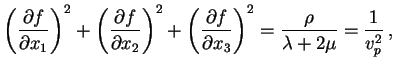
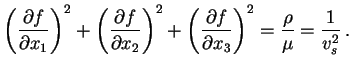
As a check, I set the elasticity matrix equal to the isotropic elasticity matrix in terms of $\lambda$ and $\mu$ and evaluated the determinant with Mathematica and set it equal to zero to get

$$\left\{(\lambda+2\mu)\left[\left(\frac{\partial f}{\partial x_1}\... ...}\right)^2 +\left(\frac{\partial f}{\partial x_3}\right)^2\right]\right\}=0 ,$$

which leads to

$$\left(\frac{\partial f}{\partial x_1}\right)^2 +\left(\frac{\part... ...partial f}{\partial x_3}\right)^2= \frac{\rho}{\lambda+2\mu}=\frac{1}{v_p^2} ,$$ (12)

or

$$\left(\frac{\partial f}{\partial x_1}\right)^2 +\left(\frac{\part... ...t(\frac{\partial f}{\partial x_3}\right)^2=\frac{\rho}{\mu}= \frac{1}{v_s^2} .$$ (13)

These are the eikonal equations for P and S waves in isotropic inhomogeneous media; thus the material in appendices A and B is not demonstrated to be incorrect. However, the determinant in appendix B seems a bit long, so I will triple-check for typos before attempting numerical solution.